Assessing Street Vegetation Rate in NYC
\ Abstract
This project examines street-level vegetation visibility in Manhattan, New York City. We obtained imagery through the Google Street View Static API, applied a pretrained ENet semantic segmentation model, and explored associations between image-derived vegetation ratios and neighborhood socioeconomic characteristics at the census-tract level.
My contribution: Within our five-person team, I focused on image segmentation: applying a pretrained ENet model with OpenCV, calculating vegetation and terrain pixel ratios, and producing segmentation visualizations. This work supported the team’s subsequent spatial mapping and statistical analysis. The case study below presents the broader team project.
Key Words: Street view imagery, Efficient neural network, Green space, Machine learning, Socioeconomic status.
GSAPP, Columbia University
Instructor: Boyeong Hong
Collaborator: Yingjie Liu, Rae Lei, Jiayi Zhao, Shuhua Li
March 2022 - May 2022
\ Introduction
Covid-19 has brought many challenges to New York City. During this turbulent time, compared with staying indoors, people tend to spend more time in outdoor green spaces while keeping a safe social distance. More than ever, New Yorkers rely on parks and other outdoor green spaces, like plazas or natural landscapes, to support their physical and mental health. Within this context, we focused on street vegetation as a visible part of everyday public-space experience.
Another benefit of street green spaces is that it is the most extensive, interconnected network of public spaces in our cities. The fabric of street networks give them great potential to become a citywide, resilient ecosystem contributing to personal wellness and the health of the natural environment. According to this streetscape design project by Gensler(Theeuwes, 2021), this expansive network street can provide protection against the effects of climate change. Gensler describes streets as accounting for roughly 30–35% of a city’s land area; this is general urban context, rather than a measurement produced by our Manhattan study.
Thus, to explore the current street vegetation condition, this project will explore the street-level vegetation visibility in Manhattan by analyzing the street view photos and neighborhood features. Through various machine learning methods, we aim to find the answers to the questions listed below:
1.Which neighborhood characteristics are most strongly associated with the street-level vegetation ratio? For instance, English proficiency, population count of specific age groups or median household income.
2.How does the street-level vegetation ratio vary across census tracts in Manhattan?
3.What kinds of urban design strategies or policies can be applied according to the analysis result?
\ Literature Review
2.1 Using machine learning to examine street green space types at a high spatial resolution: Application in Los Angeles County on socioeconomic disparities in exposure

Fig 1.Image Segmentation Source:(Sun et al., 2021)
Compared with using satellite images, “Using machine learning to examine street green space types at a high spatial resolution: Application in Los Angeles County on socioeconomic disparities in exposure” uses street-view images to calculate the green ratio in an area, which could capture different types of green spaces, like vegetation or terrain. This provides a street-level view of visible greenery that complements satellite-derived measures, although it does not directly measure people’s perceptions. And in this paper, green spaces are divided into three different types, respectively, tree, low-lying vegetation and grass. This paper has a clear structure from obtaining street-view images and training the model to the final GLMMs examination. Firstly, this team obtained socioeconomic factors online. Then, download dataset images for training models and street view images in Los Angeles. Thirdly, using semantic segmentation to measure total and types of green space. Fourthly, using Intersection over union to evaluate the performance. Fifthly, using Normalized difference vegetation index to compare the green space with satellite imagery-based green space. Finally, using generalized linear mixed models to examine the association between SES factors and street green space level. Results show that the deep learning model has a high accuracy, with 92.5% mean intersection over union. Also, three kinds of green space have negative associations with neighborhood SES. In conclusion, both the workflow of this paper and the machine learning models it used are of great reference value.
2.2 Machine learning on high performance computing for urban greenspace change detection: satellite image data fusion approach

Fig 2.Steps in green space assessment Source:(More, 2020)
Fast-changing urban regions require continuous and fast green space change detection. So This study uses a fusion approach to detect the urban greenspace change in Mumbai. This study involves satellite image classification using SVM and spatio-spectral fusion of satellite image data. It uses 4 steps, which is Pre-processing, general information and mathematics, support vector machine and spectral fusion approach for classification.
As shown in Figure2. Classification is performed on the fused data using the SVM to monitor green space changes over a period of 15 years. Results show the decreasing tendency in Mumbai, and this research concludes that good performance is achieved using machine learning for green space analysis with a spatio-spectral fusion approach.
This study illustrates a complementary approach to urban green-space assessment using satellite imagery and machine learning, rather than a method implemented in our street-view analysis.
\ Data & Methods

Fig 3.Methodology Framwork
3.1 Study Population
This project focuses on Manhattan, one of New York City’s five boroughs. Its dense urban environment and varied neighborhood conditions provide a setting for exploring how street-level vegetation visibility varies across census tracts and relates to socioeconomic characteristics.
3.2 Street View Images
We used Google Street View Static API to request the street view images as the study imagery. The API returns a static view from available Street View imagery, with the viewing direction controlled by request parameters. In the process of single image request and response, the view point is defined with URL parameters including location, fov, heading, pitch and radius and the street view picture is sent as a response through a standard Http request.(Google, n.d.)
A street-network GIS shapefile was used to define sampling locations. The sampling viewpoints were selected from streetnet through 3D visual programming platform Rhino and its plugin, Grasshopper. The plugin Urbano was used to import GIS shapefile information to the Grasshopper environment. And the plugin Kangaroo was used to decrease overlapping points. We obtained street view points and its GIS location information was used to request for street view images. In the practice, the images with heading of 0,90,180,270 and fov of 90 was selected.
3.3 social and neighborhood conditions current
To explore the current socio economic condition of neighborhoods, we downloaded a series of csv files with geoid from the US census database(U.S. Census Bureau, n.d.), including occupied housing units, median household income, monthly housing cost, total population, population of different age groups and enthnic groups, disability rate and education level(U.S. Census Bureau, n.d.).
3.4 machine learning model
We used a pretrained ENet (Efficient Neural Network) model for pixel-wise semantic segmentation. Introduced by Paszke et al. (2016), ENet was designed for low-latency processing with relatively modest computational requirements. In this project, we used the existing model for inference without training or fine-tuning its weights.
The ENet has the ability to distinguish the list of classes (Automatic Addison,2021):
Unlabeled, Road, Sidewalk, Building, Wall, Fence, Pole, TrafficLight, TrafficSign, Vegetation, Terrain, Sky, Person, Rider, Car, Truck, Bus, Train, Motorcycle, Bicycle.
We selected this pretrained model to make image processing feasible within the project’s data volume and hardware constraints.
3.5 Methodological framework
As shown in Figure 3, we developed our framework according to the literature review indicated in figure 3. The whole structure is divided into 2 parts. In the machine learning part, 2000 points were selected from the street network in Manhattan(NYC Open Data, n.d.), and their location data was extracted in GIS as an URL parameters for google street view api to get street view images. Each viewpoint requested 4 pictures in four different directions. In the meantime, we used the Efficient Neural Network model to identify vegetation and terrain through pixel-wise semantic segmentation. Later we imported all the images we had into the pre-trained model and exported the ratio of selected classes pixel by total pixel amount to calculate image-level vegetation and terrain ratios.
For the analysis stage, the image-derived ratios were grouped and averaged by census tract, then joined to neighborhood characteristics using GEOID. We used LiDAR-derived land-cover maps as a qualitative spatial comparison. After standardizing the data and filtering redundant predictors, we compared three regression models to explore associations between vegetation ratios and neighborhood characteristics.
\ Image Processing
To define sampling locations, we imported the street-network shapefile and extracted more than 10,000 street vertices (Figure 4). Requesting four views at each point would produce around 40,000 images, so we used Grasshopper to remove duplicate points and points that were too close together. This reduced the sampling locations to approximately 2,000. We then exported their coordinates, as shown in Table 1.
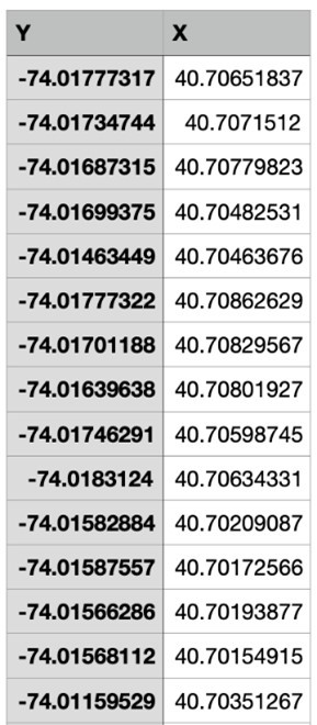
Table 1. Coordination of points
After we have all the points, we imported the lat and lon of each point into google street view api to get the images we need for further analysis as shown in figure 5.


Fig 4. Street network and vertices


Fig 5. Static street view images
We used semantic segmentation to calculate image-level vegetation and terrain ratios. First, we resized and normalized the street-view images into a four-dimensional input tensor, or blob. We passed this input to the pretrained ENet model, obtained per-pixel class scores, and assigned each pixel its highest-scoring label. We then produced a color-coded segmentation overlay and class legend (Figure 6), and calculated the percentage of pixels labeled vegetation or terrain for subsequent analysis.

Fig 6. Image segmentation and legend
Vegetation and terrain are distinct model classes. Under the Cityscapes definitions, vegetation includes trees and hedges, while terrain includes grass as well as soil and sand; terrain is therefore not a pure measure of greenery. We imported the ratio CSV into QGIS as a point layer and used a point-in-polygon operation to aggregate the measurements by census tract. The tract-level averages were then joined to 21 neighborhood characteristics, as shown in Figure 7 and Table 2.


Fig 7. Terrain and vegetation rate of each census tract

Table 2. Vegetation rate with GEOID
\ LiDAR Comparison
To compare street-level visibility with top-down land cover, we used the 2017 LiDAR-derived land-cover dataset. This raster dataset has a 6-inch resolution and was developed as part of an updated urban tree-canopy assessment (NYCDOITT, 2017). We imported the data into ArcGIS and aggregated land-cover measurements within census-tract boundaries.
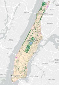
Fig 8. LiDAR Land Cover Map
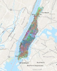
Fig 9. LiDAR Land Cover Map splitted by census tracts
We selected the Tree Canopy and Grass/Shrubs classes from the land-cover dataset. For each census tract, we divided their combined pixel count by the total count across all land-cover classes, then exported the resulting green-cover ratios to a CSV file.

Fig 10. Classes of LiDAR Land Cover dataset

Fig 11. Green ratios with GEOID based on LiDAR Land Cover Map
We created a census-tract choropleth map of the LiDAR-derived green-cover ratio and compared it visually with the street-view vegetation and terrain maps. The maps show some similar spatial patterns, but they measure different aspects of the environment: land-cover area from above and visible pixels from street level. This comparison provides context for interpretation rather than a quantitative validation of segmentation accuracy.


Fig 12. Green ratios of each census tract based on LiDAR Land Cover Dataset
Fig 13. Terrain and vegetation rate of each census tract based on street view model
\ Results
In the visual comparison, the street-view vegetation map appeared more similar to the LiDAR-derived green-cover map than the terrain map did. We use these maps as complementary views of Manhattan’s greenery, while recognizing their different perspectives and measurement definitions.
4.1 Associations between greenery rate and neighborhood features
Moving forward, we used three regression approaches and a decision-tree regressor to explore associations between greenery rate and neighborhood features. We first used seaborn heatmap to show the correlations between different features as our preliminary analysis, to identify potentially redundant predictors.
And we found there's a high correlation between predictor variables. The correlation between monthly housing costs and median household income, total population and occupied housing units are higher than 0.8. We deleted one of the pairs of these data and got the correlation matrix changes from left to the right as shown in figure 14.

Fig 14. correlation matrix
We compared OLS, Ridge, and Lasso regression. OLS showed the strongest fit in our exploratory comparison, although overall model fit remained limited. We also used a decision-tree regressor to examine the relative importance of the included features (Figure 15). These importance scores describe the fitted model; they do not establish causality or the direction of an association.

Fig 15. Feature importance
\ Implications
4.2.1.Distribution inequality
In the sampled street-view imagery, census tracts around Central Park and along the riverside generally show higher vegetation ratios. Uptown also appears greener than downtown, while Midtown shows relatively low values. These are descriptive patterns in the tract-level maps, rather than measurements of every street or resident’s exposure.
These patterns suggest an uneven distribution of visible street vegetation and identify areas for closer investigation.
4.2.2.Association with housing cost
Median monthly housing cost had the highest importance in the fitted decision-tree model, while the correlation analysis indicated a negative association with the vegetation ratio across the studied census tracts. These results do not explain why the association occurs or establish effects on residents’ health. Other neighborhood conditions may also influence the observed pattern.
4.2.3.Associations with demographic characteristics
‘Population 60 years and over’ and ‘females enrolled in school’ have positive correlation with green ratio, and these two features also have more importance from the analysis of decision tree regressor. These are tract-level associations between vegetation ratios and population counts; they do not establish individuals’ access to greenery or the reasons for the observed pattern.
In addition, ‘Percentage Population 16 years and over unemployed’ is negatively correlated with the green ratio. This association suggests a question for further equity-focused investigation; it does not establish a causal relationship between unemployment and greenery.
4.2.4 Implications
The observed variation can inform discussions about more equitable access to urban greenery. Planning decisions should also consider neighborhood needs, accessibility, and the quality of public space. Our analysis does not directly measure health outcomes or establish how much green space particular demographic groups need.
The vegetation-ratio map can help identify candidate areas for site visits and further assessment before proposing greening interventions.
\ Limitations & Future Work
5.1 Project limitations
The LiDAR comparison was visual and did not quantify segmentation accuracy against manually labeled street-view images. Predictions may contain classification errors, and the terrain class also includes non-vegetated surfaces. Image-based visibility does not fully represent human perception, accessibility, or the experience of being in a neighborhood.
In addition, the study area of this model only covers Manhattan district because of the large dataset and computing limitations. The result of this model can only explain the situations within the Manhattan area, and may not have enough data to well-explain the situation in other places.
Parks usually have a higher green ratio, which will affect our neighborhoods' correlation analysis.
5.2 Opportunities and Improvements for future analysis
For further analysis, this workflow could be evaluated in other cities and countries to explore whether similar associations are observed, with local validation before drawing planning conclusions. Future research could also include appropriate physical and mental health data. For example, New York’s land-surface temperature map could support an investigation of the relationship between vegetation visibility and heat exposure (USGS, 2019).
In addition, a mental-health services map could describe service availability, but assessing relationships between greenery and mental health would require appropriate health-outcome data and a study design that addresses confounding. (NYC Open Data, 2022) Additional datasets could support further investigation of greenery, social equity, and health, while accounting for spatial dependence, measurement uncertainty, and alternative explanations.
\ References
Cordts, M., Omran, M., Ramos, S., Rehfeld, T., Enzweiler, M., Benenson, R., Franke, U., Roth, S., & Schiele, B. (2016). The Cityscapes Dataset for Semantic Urban Scene Understanding. https://www.cityscapes-dataset.com/wordpress/wp-content/papercite-data/pdf/cordts2016cityscapes.pdf
Department of City Planning. (2020). Census - Download and Metadata. Www1.Nyc.gov. https://www1.nyc.gov/site/planning/data-maps/open-data/census-download-metadata.page
Department of Information Technology & Telecommunications. (2018, December 12). Land Cover Raster Data (2017) – 6in Resolution | NYC Open Data. Data.cityofnewyork.us. https://data.cityofnewyork.us/Environment/Land-Cover-Raster-Data-2017-6in-Resolution/he6d-2qns
Google. (n.d.). Street View Static API overview. Google Developers. https://developers.google.com/maps/documentation/streetview/overview
More, N., Nikam, V. B., & Banerjee, B. (2020). Machine learning on high performance computing for urban greenspace change detection: satellite image data fusion approach. International Journal of Image and Data Fusion, 11(3), 218–232. https://doi.org/10.1080/19479832.2020.1749142
NYC Open Data. (n.d.). NYC Street Centerline (CSCL). NYC Open Data. https://data.cityofnewyork.us/City-Government/NYC-Street-Centerline-CSCL-/exjm-f27b
NYC Open Data. (2022). Mental health of NYC. Cityofnewyork.us. https://mentalhealth.cityofnewyork.us/wp-content/uploads/2021/05/CMH-MapforWebsite-scaled.jpg
NYC Open data. (2017). NYC LiDAR. Maps.nyc.gov. https://maps.nyc.gov/lidar/2017/
Ouyang, C. (Elvin). (2020, May 31). How to Query Google Street View Static API with Python (UPDATED IN 2020). Elvin Ouyang’s Blog. https://elvinouyang.github.io/project/how-to-query-google-street-view-api-with-python/
Sears-Collins, A. (2021, February 27). How To Detect Objects Using Semantic Segmentation – Automatic Addison. https://automaticaddison.com/how-to-detect-objects-using-semantic-segmentation/
Sun, Y., Wang, X., Zhu, J., Chen, L., Jia, Y., Lawrence, J. M., Jiang, L., Xie, X., & Wu, J. (2021). Using machine learning to examine street green space types at a high spatial resolution: Application in Los Angeles County on socioeconomic disparities in exposure. Science of the Total Environment, 787, 147653. https://doi.org/10.1016/j.scitotenv.2021.147653
Theeuwes, J. T. (2021, April 9). Creating Resilient Urbanism With Streetscape Design. Gensler. https://www.gensler.com/blog/creating-resilient-urbanism-with-streetscape-design
U.S. Census Bureau. (n.d.). Explore Census Data. Data.census.gov. Retrieved April 26, 2022, from https://data.census.gov/cedsci/table?g=0500000US36061%241400000&d=ACS%205-Year%20Estimates%20Detailed%20Tables
USGS. (2019). Urban Heat New York City | U.S. Geological Survey. Www.usgs.gov. https://www.usgs.gov/media/images/urban-heat-new-york-city